LSTM은 RNN(Recurrent Neural Network)의 한 종류로, 장기 의존성 문제를 해결하기 위해 개발된 모델
기본 RNN은 시간이 지남에 따라 기울기 소실(Vanishing Gradient) 문제가 발생하는데, LSTM은 셀 상태(Cell State)와 게이트 구조(Gates)를 활용하여 이를 해결
1. LSTM의 주요 구성 요소
셀 상태(Cell State): 네트워크의 장기 기억을 유지하는 경로
입력 게이트(Input Gate): 새로운 정보를 셀 상태에 추가할지 여부 결정
망각 게이트(Forget Gate): 불필요한 정보를 제거
출력 게이트(Output Gate): 현재 상태에서 어떤 값을 출력할지 결정
LSTM은 이 3가지 게이트를 통해 장기 기억을 유지하면서 시계열 데이터를 효과적으로 학습할 수 있음
2. LSTM의 수식 : 게이트 연산
LSTM의 동작을 수식으로 정리하면 다음과 같음
각 게이트는 시그모이드(𝜎) 활성화 함수를 사용하여 0~1 사이 값을 출력하고, 이는 얼마나 정보를 유지할지 결정
2.1 망각 게이트(Forget Gate)
2.2 입력 게이트(Input Gate)
2.3셀 상태 업데이트(Candidate Cell State)
2.4최종 셀 상태(Cell State)
2.5은닉 상태(hidden state) 업데이트
3. 마케팅 데이터를 활용한 시나리오
한 전자상거래 기업이 과거 3년간의 월별 매출 데이터를 기반으로 다음 달 매출을 예측하려 한다. 입력 데이터(X): 과거 12개월의 매출 출력 데이터(y): 다음 달의 매출 데이터를 LSTM 모델로 학습하여, 패턴을 찾아 매출 변동을 예측
▶ LSTM 실습 코드
import numpy as np
import pandas as pd
import tensorflow as tf
from tensorflow.keras.models import Sequential
from tensorflow.keras.layers import LSTM, Dense
from sklearn.preprocessing import MinMaxScaler
import matplotlib.pyplot as plt

# 1. 하드코딩된 마케팅 매출 데이터 (3년간 월별 매출)
data = {
    'Month': pd.date_range(start='2020-01-01', periods=36, freq='M'),
    'Sales': [
        200, 220, 250, 270, 300, 350, 400, 380, 360, 340, 310, 280,
        240, 260, 290, 310, 340, 390, 420, 400, 370, 350, 320, 290,
        260, 280, 310, 330, 360, 410, 440, 420, 390, 370, 340, 310
    ]
}

df = pd.DataFrame(data)
df.set_index('Month', inplace=True)

# 2. 데이터 정규화
scaler = MinMaxScaler(feature_range=(0, 1))
df_scaled = scaler.fit_transform(df)

# 3. LSTM 입력 데이터 생성 (과거 12개월 -> 다음 달 예측)
def create_sequences(data, seq_length=12):
    X, y = [], []
    for i in range(len(data) - seq_length):
        X.append(data[i:i+seq_length])
        y.append(data[i+seq_length])
    return np.array(X), np.array(y)

seq_length = 12
X, y = create_sequences(df_scaled, seq_length)

# 4. 학습 데이터와 테스트 데이터 분할 (80% 학습, 20% 테스트)
train_size = int(len(X) * 0.8)
X_train, X_test = X[:train_size], X[train_size:]
y_train, y_test = y[:train_size], y[train_size:]

# 5. LSTM 모델 구축
model = Sequential([
    LSTM(50, activation='relu', input_shape=(seq_length, 1), return_sequences=True),
    LSTM(50, activation='relu'),
    Dense(1)
])

# 6. 모델 컴파일
model.compile(optimizer='adam', loss='mse')

# 7. 모델 학습
history = model.fit(X_train, y_train, epochs=100, batch_size=16, validation_data=(X_test, y_test))

# 8. 예측 수행
y_pred = model.predict(X_test)

# 9. 결과 되돌리기 (Inverse Transform)
y_test_inv = scaler.inverse_transform(y_test.reshape(-1, 1))
y_pred_inv = scaler.inverse_transform(y_pred)

# 10. 결과 시각화
plt.figure(figsize=(12, 6))
plt.plot(df.index[-len(y_test):], y_test_inv, label="Actual Sales", marker="o")
plt.plot(df.index[-len(y_test):], y_pred_inv, label="Predicted Sales", linestyle="--", marker="s")
plt.xlabel("Month")
plt.ylabel("Sales")
plt.title("LSTM Marketing Sales Prediction")
plt.legend()
plt.show()
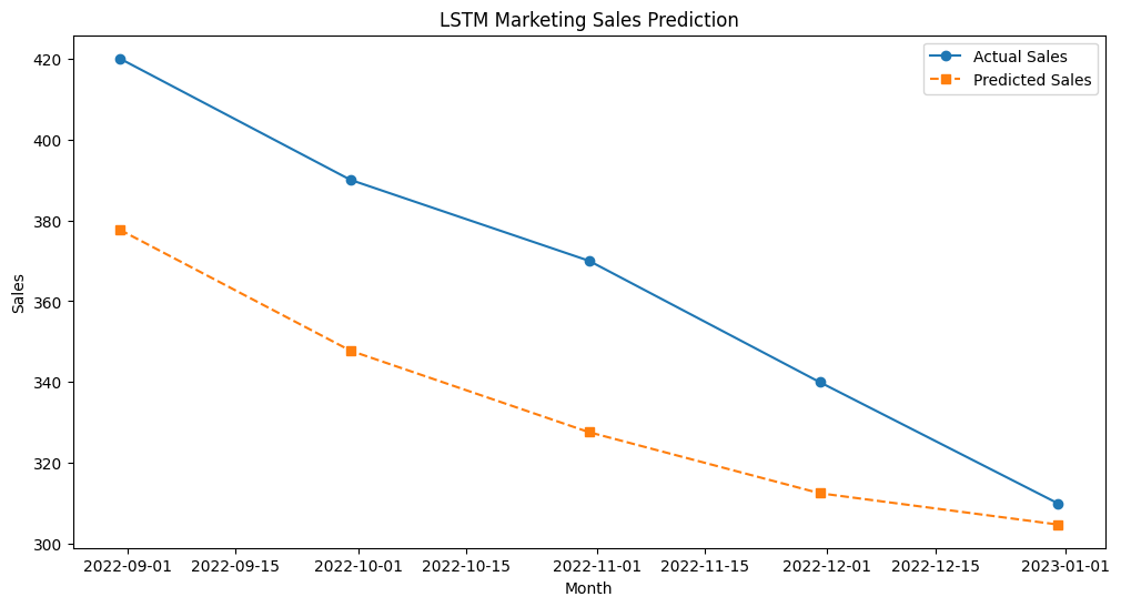
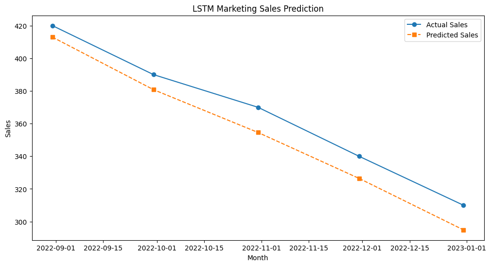
▶ 출력 결과 (최적의 파라미터 찾기)
epochs = 100
epochs = 1000
LSTM 모델 성능평가
이론 내용 중복 생략
1. 마케팅 데이터를 활용한 성능평가 시나리오
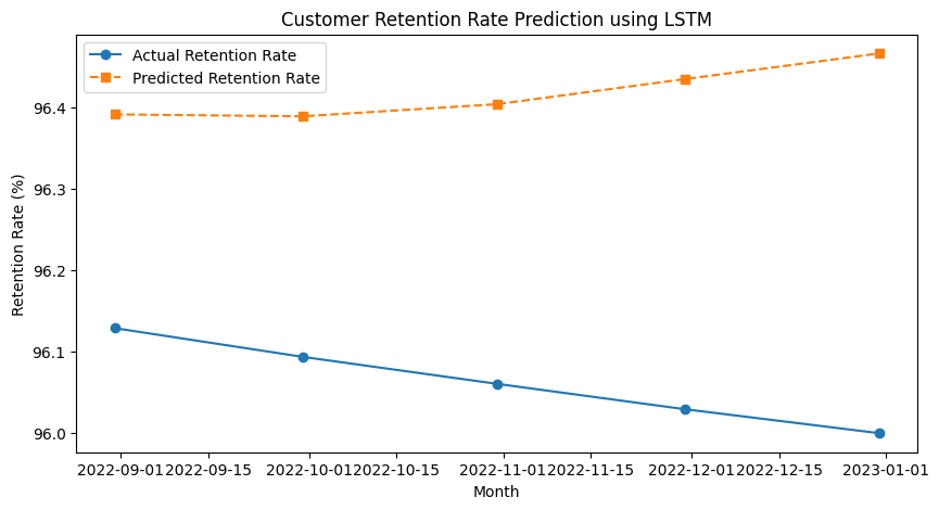
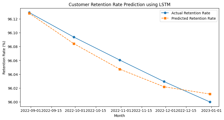
1.1 고객 유지율 예측 (Customer Retention Prediction)
시나리오 한 SaaS(Software as a Service) 기업은 고객 유지율(retention rate)을 예측하고자 한다. 이 기업은 매월 구독자의 수와 이탈 고객 수를 기록하여 고객 유지율을 분석한다. LSTM 모델을 사용하여 다음 달의 고객 유지율을 예측하고, 이를 기반으로 마케팅 전략을 수립한다.
1.2 광고 캠페인 성과 예측 (Ad Campaign Performance Prediction)
시나리오 전자상거래 회사는 페이스북과 구글에서 광고를 진행하며, 월별 광고비와 매출 데이터를 기반으로 광고 성과를 예측하고자 한다. LSTM 모델을 사용하여 다음 달의 광고 투자 대비 매출 성과(ROAS, Return on Ad Spend)를 예측한다.
▶코드 예제
# 1. 데이터 정의
data = {
    'Month': pd.date_range(start='2020-01-01', periods=36, freq='M'),
    'Ad Spend': np.linspace(50, 150, 36) + np.random.randn(36) * 5,  # 광고비 (만원)
    'Revenue': np.linspace(100, 300, 36) + np.random.randn(36) * 10  # 광고 매출 (만원)
}
df = pd.DataFrame(data)
df['ROAS'] = df['Revenue'] / df['Ad Spend']
df.set_index('Month', inplace=True)

# 2. 데이터 정규화 및 LSTM 적용
scaler = MinMaxScaler()
df_scaled = scaler.fit_transform(df[['ROAS']])
X, y = create_sequences(df_scaled, seq_length=12)
train_size = int(len(X) * 0.8)
X_train, X_test, y_train, y_test = X[:train_size], X[train_size:], y[:train_size], y[train_size:]

# 3. 모델 학습 및 예측
model.fit(X_train, y_train, epochs=100, batch_size=16, validation_data=(X_test, y_test))
y_pred = model.predict(X_test)

# 4. 예측 결과 시각화
y_test_inv = scaler.inverse_transform(y_test.reshape(-1, 1))
y_pred_inv = scaler.inverse_transform(y_pred)

plt.figure(figsize=(10, 5))
plt.plot(df.index[-len(y_test):], y_test_inv, label="Actual ROAS", marker="o")
plt.plot(df.index[-len(y_test):], y_pred_inv, label="Predicted ROAS", linestyle="--", marker="s")
plt.xlabel("Month")
plt.ylabel("ROAS")
plt.title("Ad Campaign Performance Prediction using LSTM")
plt.legend()
plt.show()
▶코드 결과 (최적의 파라미터 찾기)
epochs = 100
epochs = 1000
"오늘의 회고"
오늘은 갑근 강사님의 마지막 수업 시간 이었다. 부트캠프 시작한지 그리 오래되지 않은 것 같은데 새삼 실감이 나고 아쉽기도 하고 그간 참여 하던 내 태도도 되돌아보는 하루 였다. 길것만 같던 시간 이었는데 이렇게 빨리 가는 걸 보니 남은 기간도 금방 지나갈 것 같아 불안해지기도 했다. 지난 데이터에 관한 수업들 복습도 잘하고 또 새로운 강사님과 함께하는 수업도 집중해서 참여해야겠다..!!